魔域位列混沌优化算法(COA):从理论到实践的探索之旅
混沌理论揭示了确定性系统中隐藏的复杂性和不可预测性,魔域位列而混沌优化算法正是借鉴了混沌系统对初始条件的敏感性、遍历性和内在的随机性,通过模拟混沌动态过程来探索优化问题的解空间。
这种算法不仅能够有效避免陷入局部最优,还能在全局范围内高效搜索,展现出强大的适应性和灵活性。
今天,我们要揭开这个神秘而强大的智能优化算法的面纱——混沌优化算法。
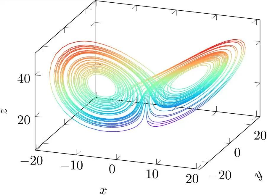
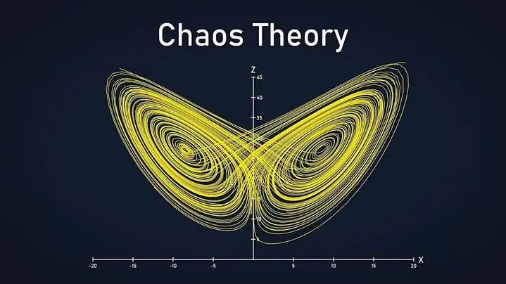
一、混沌理论的魅力提到混沌,你可能会想起蝴蝶效应——一只蝴蝶在巴西扇动翅膀,可能会在美国德克萨斯州引发一场龙卷风。

这个看似荒诞不经的比喻,正是混沌理论的核心特征之一:初始条件的敏感性。
混沌系统对初始条件极为敏感,即使微小的差异也会在迭代过程中被迅速放大,最终导致截然不同的结果。
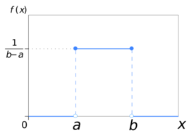
但混沌并非完全无序。它具有一种独特的“伪随机性”和“遍历性”。
混沌系统虽然看似杂乱无章,但其运动轨迹却能在整个可行空间内均匀分布,且不会重复经过同一个点。
这种特性使得混沌系统在搜索过程中能够高效地探索整个解空间,避免陷入局部最优。
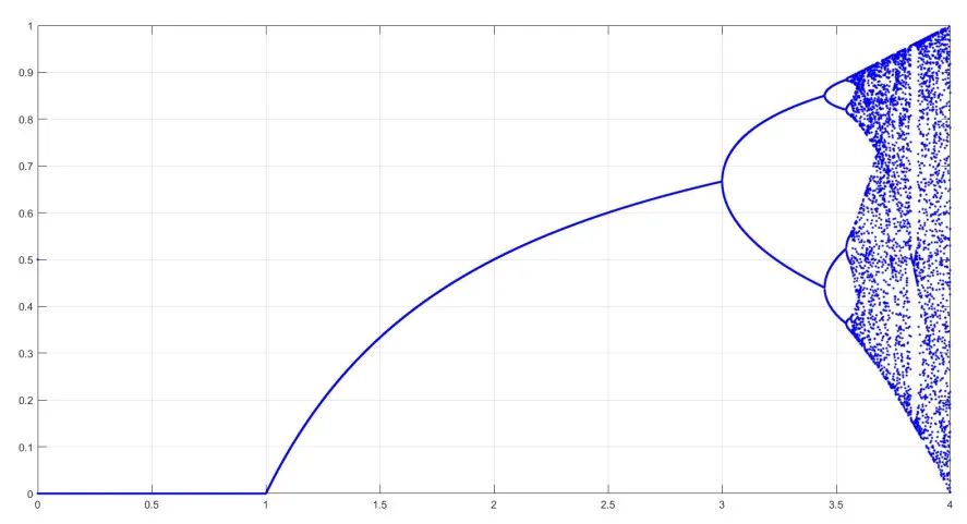
▲ Logistic混沌映射的分叉图
混沌映射是混沌理论在优化算法中的重要应用。常见的混沌映射有Logistic映射和Tent映射。
Logistic映射是一个简单的非线性方程,其迭代过程却能产生复杂的混沌行为。
Tent映射则以其线性分段的特性,展现出快速的遍历性和良好的随机性。
这些混沌映射为混沌优化算法提供了强大的动力源泉。
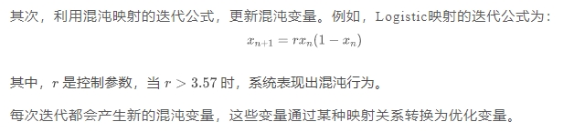
二、混沌优化算法的原理与流程混沌优化算法的核心思想是将混沌变量引入优化问题的变量空间,利用混沌运动的遍历性来搜索全局最优解。
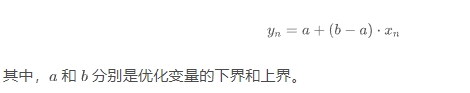
它通过混沌映射生成混沌变量,这些变量在迭代过程中不断变化,从而驱动优化变量在解空间中进行高效的搜索。
混沌优化算法的实现步骤如下:
1.初始化混沌变量首先,根据优化问题的规模和维度,初始化混沌变量。
这些变量通常在[0,1]区间内均匀分布,通过混沌映射进行迭代更新。
将转换后的优化变量代入目标函数,计算其适应度值。
根据适应度值的大小,选择最优解作为当前迭代的候选解。
4.终止条件判断最后,当达到预设的迭代次数或适应度值收敛时,算法终止,输出全局最优解。
三、混沌优化算法的案例演示为了更好地理解混沌优化算法的工作原理,我们以Ackley函数为例进行优化。
1.问题定义Ackley函数是一个经典的多峰函数,具有复杂的地形和多个局部最小值,常用于测试优化算法的性能。
import numpy as np import matplotlib.pyplot as plt from mpl_toolkits.mplot3d import Axes3D from matplotlib.animation import FuncAnimation from IPython.display import HTML import time import math # 设置中文显示 plt.rcParams['font.sans-serif'] = ['SimHei'] plt.rcParams['axes.unicode_minus'] = False # Ackley函数 defackley(x): a = 20 b = 0.2 c = 2 * np.pi d = len(x) sum_sq = sum([xi**2for xi in x]) sum_cos = sum([np.cos(c * xi) for xi in x]) term1 = -a * np.exp(-b * np.sqrt(sum_sq / d)) term2 = -np.exp(sum_cos / d) return term1 + term2 + a + np.exp(1)
2.算法建模在实现混沌优化算法时,我们选择了Logistic混沌映射作为混沌序列的生成方式。
# Logistic混沌映射 deflogistic_map(x, mu=4.0): return mu * x * (1 - x) # 混沌优化算法 defchaos_optimization(obj_func, dim, lb, ub, max_iter, chaos_iter=1000): """ 参数: - obj_func: 目标函数 - dim: 问题维度 - lb: 下界 - ub: 上界 - max_iter: 最大迭代次数 - chaos_iter: 混沌迭代次数 """ # 初始化混沌变量 chaos_vars = np.random.rand(dim) # 生成混沌序列 chaos_sequence = [] for _ inrange(chaos_iter): chaos_vars = logistic_map(chaos_vars) chaos_sequence.append(chaos_vars.copy()) chaos_sequence = np.array(chaos_sequence) # 将混沌序列映射到搜索空间 search_points = lb + (ub - lb) * chaos_sequence # 评估初始解 fitness = np.array([obj_func(p) for p in search_points]) best_idx = np.argmin(fitness) best_position = search_points[best_idx].copy() best_fitness = fitness[best_idx] # 记录历史 history = { 'positions': [search_points.copy()], 'best_position': [best_position.copy()], 'best_fitness': [best_fitness], 'current_iter': [0] } # 算法开始 print("="*50) print("混沌优化算法(COA)开始运行") print(f"搜索空间维度: {dim}") print(f"搜索范围: [{lb}, {ub}]") print(f"最大迭代次数: {max_iter}") print(f"混沌迭代次数: {chaos_iter}") print(f"初始最佳适应度: {best_fitness:.6f}") print("="*50) time.sleep(1) # 二次载波搜索 foriterinrange(max_iter): # 缩小搜索范围 current_lb = np.maximum(lb, best_position - (ub - lb) * 0.9**(iter+1)) current_ub = np.minimum(ub, best_position + (ub - lb) * 0.9**(iter+1)) # 生成新的混沌序列 new_chaos_vars = np.random.rand(dim) new_search_points = [] for _ inrange(chaos_iter): new_chaos_vars = logistic_map(new_chaos_vars) new_point = current_lb + (current_ub - current_lb) * new_chaos_vars new_search_points.append(new_point) new_search_points = np.array(new_search_points) # 评估新解 new_fitness = np.array([obj_func(p) for p in new_search_points]) current_best_idx = np.argmin(new_fitness) current_best_position = new_search_points[current_best_idx].copy() current_best_fitness = new_fitness[current_best_idx] # 更新最优解 if current_best_fitness < best_fitness: best_position = current_best_position.copy() best_fitness = current_best_fitness # 记录历史 history['positions'].append(new_search_points.copy()) history['best_position'].append(best_position.copy()) history['best_fitness'].append(best_fitness) history['current_iter'].append(iter+1) # 打印进度 ifiter % 10 == 0oriter == max_iter-1: print(f"迭代 {iter+1:3d}/{max_iter} | 当前最佳适应度: {best_fitness:.6f}") print("="*50) print("优化完成!") print(f"找到的最佳解: {best_position}") print(f"最佳适应度值: {best_fitness:.6f}") print("="*50) time.sleep(1) print("生成可视化结果...") time.sleep(1) return history
3.结果可视化为了更直观地展示混沌优化算法的优化过程,我们通过Matplotlib绘制了3D曲面图、2D等高线图和收敛曲线。
# 参数设置 dim = 2 lb = -5 ub = 5 max_iter = 50 chaos_iter = 500 # 运行算法 history = chaos_optimization(ackley, dim, lb, ub, max_iter, chaos_iter) # 准备可视化数据 x = np.linspace(lb, ub, 100) y = np.linspace(lb, ub, 100) X, Y = np.meshgrid(x, y) Z = np.zeros_like(X) for i inrange(X.shape[0]): for j inrange(X.shape[1]): Z[i,j] = ackley([X[i,j], Y[i,j]]) # 创建可视化图形 fig = plt.figure(figsize=(18, 6), dpi=100) fig.suptitle('混沌优化算法优化过程', fontsize=16) # 统一子图尺寸 gs = fig.add_gridspec(2, 3, width_ratios=[1, 1, 1], height_ratios=[1, 1]) # 3D曲面图 ax1 = fig.add_subplot(gs[:, 0], projection='3d') surf = ax1.plot_surface(X, Y, Z, cmap='viridis', alpha=0.6) fig.colorbar(surf, ax=ax1, shrink=0.6, aspect=10, label='函数值') scatter = ax1.scatter([], [], [], c='red', s=10, alpha=0.5, label='混沌搜索点') best_scatter = ax1.scatter([], [], [], c='blue', marker='*', s=200, label='最优解') ax1.set_title('3D函数曲面与混沌搜索', fontsize=12) ax1.set_xlabel('x1', fontsize=10) ax1.set_ylabel('x2', fontsize=10) ax1.set_zlabel('f(x)', fontsize=10) ax1.legend(loc='upper right', fontsize=8) # 2D等高线图 ax2 = fig.add_subplot(gs[:, 1]) contour = ax2.contourf(X, Y, Z, levels=50, cmap='viridis') fig.colorbar(contour, ax=ax2, shrink=0.6, aspect=10, label='函数值') scatter2d = ax2.scatter([], [], c='red', s=10, alpha=0.5, label='混沌搜索点') best_scatter2d = ax2.scatter([], [], c='blue', marker='*', s=100, label='最优解') search_area = plt.Rectangle((0,0), 0, 0, color='yellow', alpha=0.3, label='当前搜索区域') ax2.add_patch(search_area) ax2.set_title('2D等高线与混沌搜索', fontsize=12) ax2.set_xlabel('x1', fontsize=10) ax2.set_ylabel('x2', fontsize=10) ax2.legend(loc='upper right', fontsize=8) # 收敛曲线 ax3 = fig.add_subplot(gs[0, 2]) convergence_line, = ax3.plot([], [], 'b-', linewidth=2, label='最佳适应度') current_point = ax3.scatter([], [], c='red', s=50, label='当前值') ax3.set_title('适应度收敛曲线', fontsize=12) ax3.set_xlabel('迭代次数', fontsize=10) ax3.set_ylabel('适应度值', fontsize=10) ax3.grid(True, linestyle='--', alpha=0.6) ax3.set_xlim(0, max_iter) ax3.set_ylim(0, max(history['best_fitness'])) ax3.legend(loc='upper right', fontsize=8) # 参数显示 ax4 = fig.add_subplot(gs[1, 2]) ax4.axis('off') info_text = ax4.text(0.1, 0.5, '', fontsize=10, bbox=dict(facecolor='white', alpha=0.8)) plt.tight_layout() # 修改更新函数 defupdate(frame): # 只显示部分点避免过于密集 display_points = history['positions'][frame][::10] # 更新3D图 current_z = np.array([ackley(p) for p in display_points]) scatter._offsets3d = (display_points[:,0], display_points[:,1], current_z) best_pos = history['best_position'][frame] best_z = ackley(best_pos) best_scatter._offsets3d = ([best_pos[0]], [best_pos[1]], [best_z]) # 更新2D图 scatter2d.set_offsets(display_points) best_scatter2d.set_offsets([best_pos]) # 初始化搜索区域 current_iter = history['current_iter'][frame] if current_iter == 0: # 第一帧使用全局搜索范围 current_lb = np.array([lb, lb]) current_ub = np.array([ub, ub]) else: # 后续帧缩小搜索范围 current_lb = np.maximum(lb, best_pos - (ub - lb) * 0.9**current_iter) current_ub = np.minimum(ub, best_pos + (ub - lb) * 0.9**current_iter) # 更新搜索区域显示 search_area.set_xy((current_lb[0], current_lb[1])) search_area.set_width(current_ub[0] - current_lb[0]) search_area.set_height(current_ub[1] - current_lb[1]) # 更新收敛曲线 x_data = range(current_iter+1) y_data = history['best_fitness'][:current_iter+1] convergence_line.set_data(x_data, y_data) current_point.set_offsets([[current_iter, history['best_fitness'][current_iter]]]) # 更新文本信息 info = f"迭代次数: {current_iter}\n" info += f"最佳适应度: {history['best_fitness'][current_iter]:.6f}\n" info += f"最佳位置: [{best_pos[0]:.4f}, {best_pos[1]:.4f}]\n" info += f"搜索区域: [{current_lb[0]:.2f}, {current_ub[0]:.2f}] x [{current_lb[1]:.2f}, {current_ub[1]:.2f}]\n" info += f"混沌迭代次数: {chaos_iter}\n" info += f"当前搜索点数: {len(history['positions'][frame])}" info_text.set_text(info) return scatter, best_scatter, scatter2d, best_scatter2d, search_area, convergence_line, current_point, info_text # 创建动画 ani = FuncAnimation(fig, update, frames=len(history['positions']), interval=500, blit=True) # 显示动画 plt.close() HTML(ani.to_jshtml())
经过50次迭代,混沌优化算法成功找到了Ackley函数的全局最优解。
结 语混沌优化算法以其独特的混沌理论基础、强大的全局搜索能力和广泛的应用领域,在智能优化领域展现出巨大的潜力。
它不仅能够解决复杂的优化问题,还能够与其他优化算法相结合,实现更高效的优化搜索。